
Wildlife Seasonal Modelling
The models described in this booklet explore what simple processes might give rise to the patterns seen in seasonal observations. The observed curves used throughout are derived from long-term monthly aggregation of wildlife observation records collected within the study area.
Each model begins with a small set of assumptions — about presence, detectability, and seasonal change — and asks whether these are sufficient to reproduce the curves observed in the data.
Detectability here refers to the likelihood of observing or recording a species, rather than its absolute abundance.
Across species, three distinct ways of occupying the year emerge.
Some species are present only for part of the year, appearing within a defined seasonal window before disappearing again. Others are present throughout the year, but vary in how readily they are observed, their detectability rising and falling with behaviour and conditions. A third group — winter visitors — spans the year boundary, arriving in autumn, peaking in winter, and departing in spring.
These differences suggest three complementary models:
- Seasonal presence, where activity is confined to a bounded window
- Resident detectability, where presence is continuous but visibility varies
- Winter presence, where activity wraps around the year boundary with a winter peak
Each model is deliberately simple. They do not attempt to capture ecological processes in detail, nor are they intended to predict future observations. Instead, they act as a way of testing whether the broad patterns seen in the observed data can arise from straightforward mechanisms.
The modelling workflow is illustrated below:
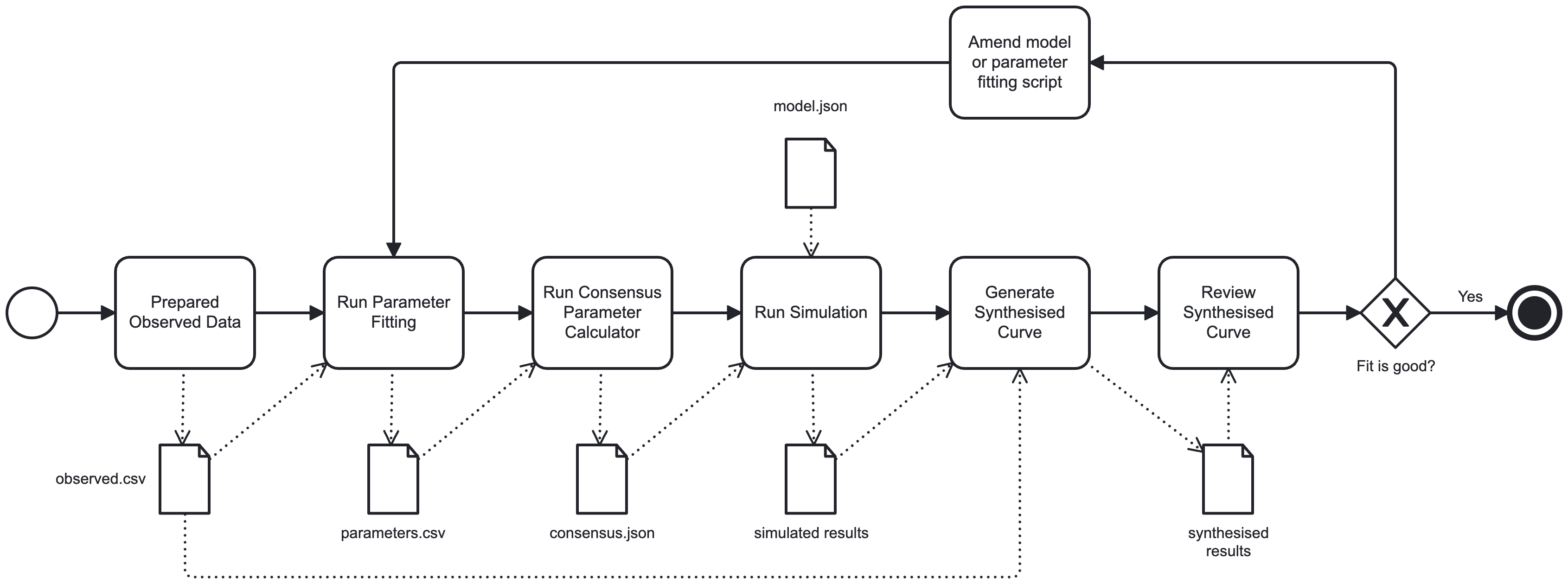
A parameter fitting process identifies a search space, defined in terms of the model parameters, and then repeatedly runs the model with parameters selected randomly from within that search space, scoring each run in terms of closeness to the observed data.
On completion, a consensus parameter set is derived from the individual sets that produced the closest matches and this is used to generate a synthesised seasonal curve, one that follows the shape of the simulated output but is scaled onto the observed data scale to allow easy comparison.
This allows each species to be described not only by its pattern, but by a small set of parameters — the consensus set — that together form a simple seasonal “signature”.
The features in that signature describe aspects of seasonal behaviour such as:
- Peak timing
- Seasonal width
- Detectability persistence
- Seasonal symmetry and asymmetry
- Occupancy characteristics
- Derived ecological traits
In this way, the models sit alongside the observations. The observations describe how species occupy the year; the models ask how those patterns might come to be, and provide a consistent way of comparing them.
Contents
| Title | Description |
|---|---|
| Resident Detectability Model | How a resident species varies in visibility through the year |
| Seasonal Presence Model | When a species appears within the year |
| Winter Visitor Model | When a species appears across the year boundary |
| Worked Example - the Bluebell | Step-by-step example showing how seasonal structure emerges from a fitted model |
| Species Similarity and Clustering | Comparisons of seasonal behaviour across species, revealing patterns of similarity |
| Ecological Neighbourhoods | Clusters of species that occupy similar regions of seasonal ecological space |
| Seasonal Ecological Calendars | Calendar-style views of seasonal activity |
| Glossary | Definitions and explanations of modelling terms, parameters, and ecological concepts |
Tool
ODE Solver
A simple tool for exploring time-based models
The seasonal presence and detectability models were developed using a small, general-purpose ordinary differential equation solver, designed for experimentation and visualisation.
It allows simple systems to be defined and explored over time, making it possible to test how patterns might arise from underlying processes.
The application, the models, and instructions on how to run them are provided in the GitHub repository.