Worked Example — Bluebell (Hyacinthoides non-scripta)

The following example illustrates how a single species moves through the modelling workflow, from observed seasonal data to fitted model, classification, and ecological neighbourhood analysis.

The purpose is not to reproduce the technical implementation in detail, but to show how the different stages of the workflow connect together interpretively.

Observed Seasonal Pattern

The starting point is the observed seasonal curve derived from long-term monthly observations.

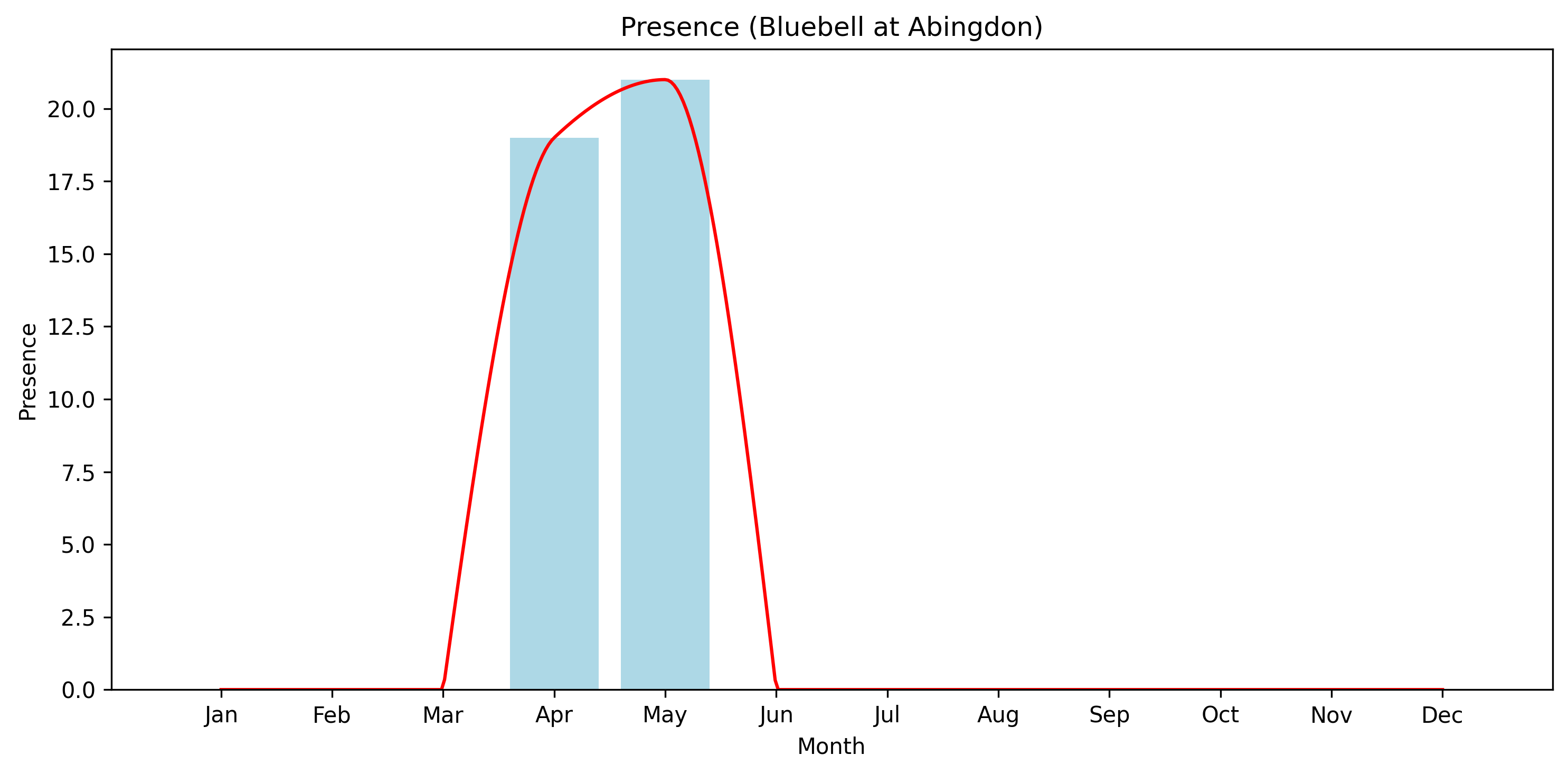
The curve shows:

• Near-absence through autumn and winter
• Rapid emergence during spring
• A sharply bounded flowering peak
• Rapid decline after the flowering period ends

This immediately suggests a strongly seasonal presence structure rather than a continuously detectable resident pattern.

Initial Classification

The observed curve is first examined using a rule-based classification stage.

The bluebell pattern shows several strongly seasonal characteristics:

• A narrow active period
• Extended absence outside the flowering season
• Strong asymmetry between emergence and decline
• Low year-round occupancy

These features place the species within the Seasonal Presence Model family.

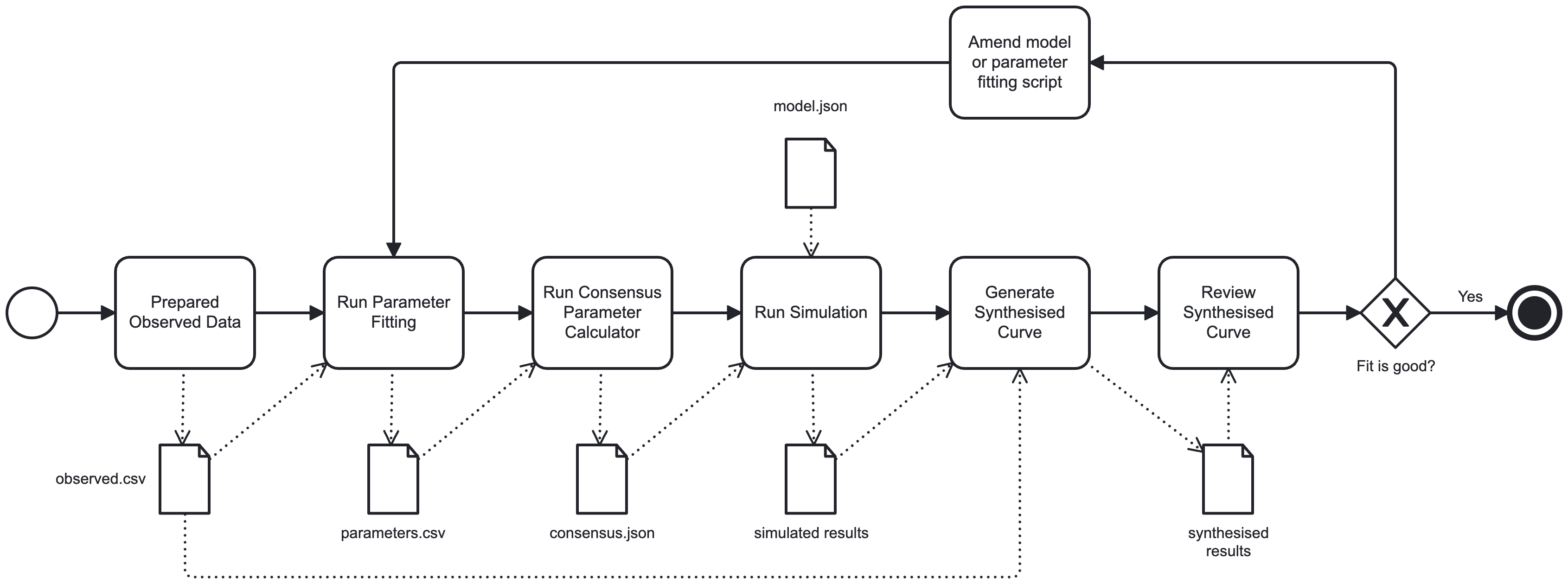
Parameter Fitting

Once a model family has been selected, the parameter fitting process begins.

A search space is constructed describing plausible ranges for:

• Seasonal onset and end
• Peak timing
• Seasonal sharpness
• Growth and decay behaviour
• Post-season suppression strength

The model is then repeatedly simulated using randomly selected parameter combinations.

Each simulation is compared against the observed curve and scored according to:

• Overall curve similarity
• Peak timing agreement
• Seasonal width agreement
• Agreement in low-activity months

The highest-scoring parameter sets are retained for further analysis.

Consensus Derivation

Rather than selecting a single “best” parameter set, the workflow derives a consensus seasonal description from multiple high-scoring simulations.

This reduces the influence of unstable individual fits and produces a more representative description of the species’ seasonal structure.

The resulting consensus parameters describe features such as:

• Approximate seasonal onset
• Seasonal duration
• Timing of peak activity
• Abruptness of post-season decline

These parameters together form a compact seasonal signature for the species.

Fitted Seasonal Curve

Using the consensus parameter set, a synthesised seasonal curve can be generated and compared directly against the observed data.

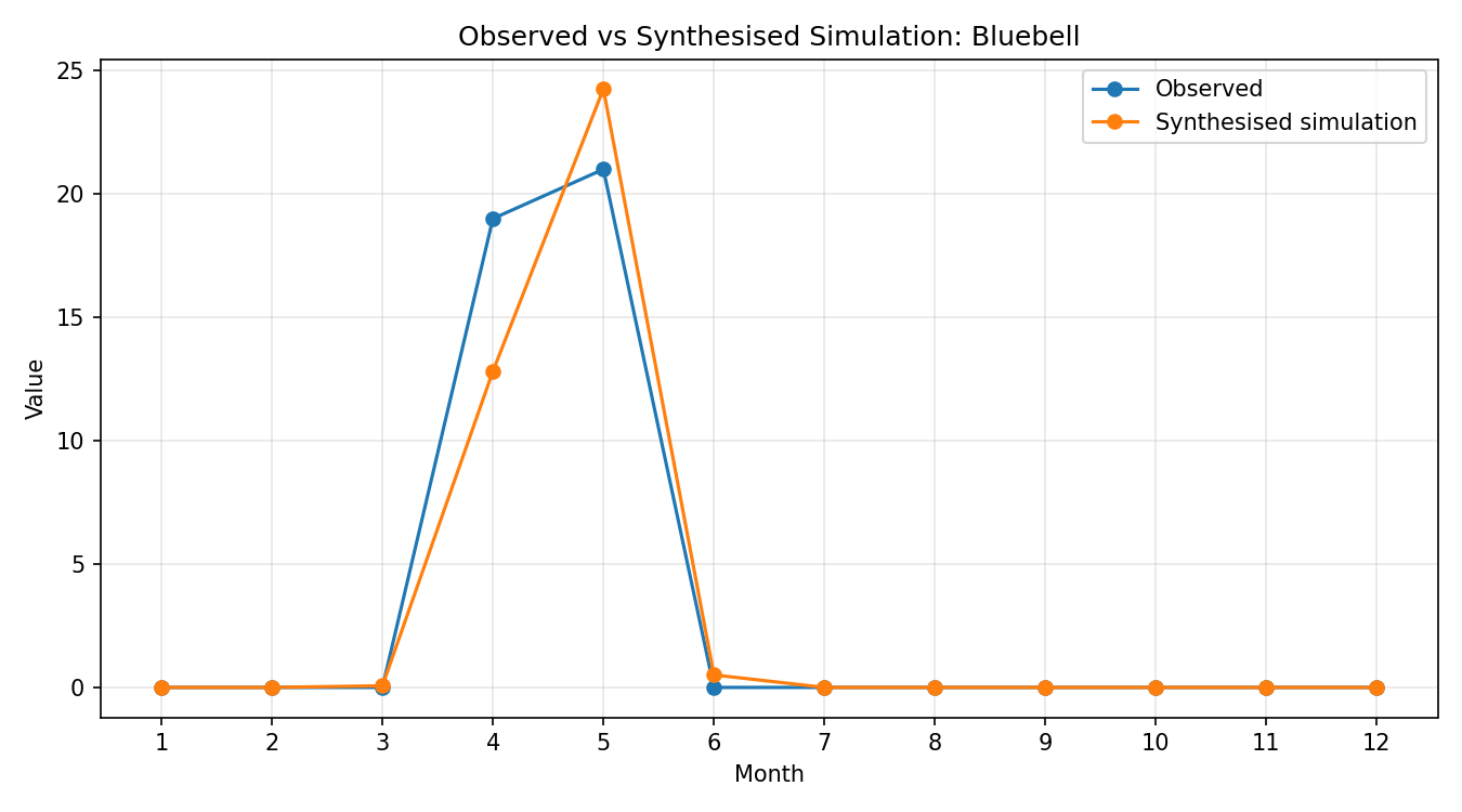
The fitted curve reproduces the main structural characteristics of the observed seasonal pattern:

• Rapid spring emergence
• A concentrated flowering peak
• Strong post-season collapse
• Extended seasonal absence

The aim is not exact prediction, but structural agreement with the observed ecological pattern.

Feature Extraction

Once fitted, the species can be represented within a broader ecological feature space.

The fitted model and observed seasonal characteristics are converted into features describing:

• Seasonal timing
• Width and concentration
• Persistence behaviour
• Occupancy structure
• Seasonal asymmetry

These features allow comparison with species from other model families using a shared seasonal representation.

Ecological Neighbourhoods

Within the resulting ecological space, bluebell clusters with species sharing similar seasonal timing and structural behaviour.

These may include:

• Other spring-flowering plants
• Species with sharply bounded emergence periods
• Species exhibiting strong seasonal concentration

The neighbourhood therefore reflects similarity of seasonal ecological structure rather than taxonomic relationship.

Interpretation

This example illustrates the broader aim of the modelling workflow.

The system does not attempt to reconstruct detailed ecological mechanisms directly. Instead, it asks whether relatively simple seasonal processes are sufficient to reproduce the large-scale structures seen in long-term observational data.

In doing so, the workflow allows species to be described not only individually, but also as components of a larger seasonal ecological landscape.