Seasonal Presence Model

The Seasonal Presence Model is designed for species whose observable appearance is strongly constrained to a limited portion of the annual cycle.

Typical examples include:

• Migratory birds
• Spring flowers
• Butterflies
• Other species with sharply bounded seasonal activity periods

Unlike the resident detectability model, which assumes continuous year-round presence, the seasonal model represents species whose observable abundance genuinely rises and falls within a restricted seasonal window.

The model forms part of the wider Wildlife Seasonal Modelling work developed for Field Notes Journal, and has also been adapted for constrained handheld systems including the TI-84 Plus CE-T Python calculator as part of the Pocket Ecology project.

Concept

The model explores whether recognisable seasonal ecological structure can emerge from a relatively small number of interacting processes rather than detailed species-specific ecological simulation.

The resulting system produces behaviours such as:

• Seasonal emergence
• Migration-driven arrival
• Flowering peaks
• Persistence through active periods
• Post-season collapse

At its core, the model combines:

• A smooth seasonal activity window
• Periodic seasonal forcing
• Dynamic decay behaviour

The interaction between these components generates seasonal curves resembling many real-world annual observation patterns.

Seasonal Activity Window

A central feature of the model is the use of a smooth seasonal activity gate.

Rather than switching a species abruptly “on” and “off”, the system uses paired logistic transitions to create:

• Gradual seasonal onset
• A bounded active period
• Smooth seasonal decline

This avoids discontinuities in the ODE system while allowing species activity to remain strongly seasonally constrained.

The resulting activity region behaves somewhat like a soft ecological window representing the period during which the species is considered seasonally active or detectable.

Seasonal Forcing

Within the active seasonal window, the model applies a periodic forcing curve based on a raised cosine annual cycle.

This provides:

• Smooth seasonal growth
• Gradual rise toward peak activity
• Continuous year-wrapping behaviour

The forcing system avoids hard annual boundaries and allows the model to transition naturally through repeated yearly cycles.

Dynamic Decay

The model also includes multiple interacting decay mechanisms.

These include:

• Baseline decay
• Enhanced out-of-season suppression
• Optional post-peak collapse behaviour

The post-peak decay system proved especially useful for representing species whose seasonal disappearance occurs substantially faster than their initial emergence.

This allows the model to produce:

• Broad spring build-up followed by rapid collapse
• Narrow flowering windows
• Sharply bounded migration periods

Ecological Interpretation

Although mathematically compact, the model often reproduces recognisable ecological structures surprisingly well.

Different parameter combinations can produce curves resembling:

• Concentrated flowering seasons
• Short migratory appearances
• Prolonged summer occupancy
• Narrow flight periods

Importantly, the system does not attempt detailed mechanistic simulation of reproduction, mortality, or movement. Instead, it focuses on the higher-level seasonal structure visible within long-term observational records.

Example: Bluebell (Hyacinthoides non-scripta)

The example below shows the Seasonal Presence Model configured for bluebell observations.

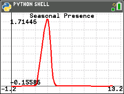
Bluebells provide a particularly suitable example for the seasonal model because their observable annual cycle is both strongly bounded and highly concentrated.

For much of the year, the species is effectively absent from observational records. During spring, however, detectability rises rapidly as flowering begins, producing a short but intense seasonal peak before collapsing again into near-zero visibility for the remainder of the year.

The model attempts to reproduce this structure using:

• A constrained seasonal activity window
• Smooth seasonal forcing
• Enhanced post-peak suppression

Several characteristic features are visible in the resulting curve:

• Rapid spring emergence
• A concentrated flowering peak
• Sharp post-peak decline
• Prolonged seasonal absence outside the active window

One of the more useful aspects of the seasonal model is its ability to represent asymmetric seasonal behaviour. In the bluebell example, emergence occurs comparatively gradually, while the post-peak decline is substantially sharper. This mirrors the observed seasonal structure of many spring woodland species whose visible phase disappears quickly following peak flowering.

Despite running on highly constrained hardware, the TI-84 implementation preserves much of the broader seasonal shape of the desktop model while carrying out all numerical integration and rendering directly on-device.

Pocket Ecology

The seasonal presence model represents an experiment in portable ecological computation:

How much ecological structure can survive when reduced to extremely small computational systems?

The resulting calculator implementation is necessarily simpler than the desktop system, but it preserves much of the seasonal behaviour and ecological interpretability of the original model while fitting inside a battery-powered handheld device originally designed for school mathematics.